 Getting your robot to obey “Go to the kitchen” seems like it should be a simple problem to solve. In fact, it requires some advanced mathematics and a lot of programming. Having ROS built into the Deep Learning Robot means that this is all available via the ROS navigation stack, but that doesn’t make it a set-and-forget feature. In this post, we’ll walk through both SLAM and autonomous navigation (derived from the Turtlebot tutorials), show you how they work, give you an overview of troubleshooting and outline the theory behind it all.
Pre-requisites
You’ll obviously need a Deep learning Robot and I’ll assume you’ve successfully followed both the Missing Instructions and the Networking Instructions. The latter in particular are key to making the demos in this post work.
I’ll also assume you’ve renamed your robot myrobot.local; simply substitute your own name in the commands below where bold is marked.
Make sure your robot is fully charged up. Strange USB communication errors start to occur with the Xtion and Kobuki when the battery is low. Plugging the robot into the power supply is not enough; the battery must actually be fully charged.
If you have a Mac, I highly recommend you set up text expansion to save you typing.
Why This is Hard
Localization is the problem in robotics that faces a robot that needs to figure out where it is on a given map using sensor data. Simultaneous Localization and Mapping (SLAM) is the more complex problem where the robot needs to figure out where it is even as it builds up a map from scratch.
Why is localization hard? After all, we have the Xtion sensor on our robot that can measure the distance to the nearest objects. We also have odometry, which I originally thought was the robot’s sense of smell but is actually a data stream from the wheel encoders that measures how many times each wheel has rotated. Finally we have the RGB video stream itself, also from the Xtion. Surely this is enough?
The problem is that none of these sources is accurate or reliable. Distance readings are noisy. The position of the robot (its “pose”) predicted by odometry quickly drifts from the real one as the wheels slip on the floor. The quality of the video stream will vary wildly under different lighting conditions. Finally, a map is only good until somebody moves a chair. Individually, none of these sound like a difficult problem but as we pile uncertainty on top of uncertainty the robot becomes totally confused.
 Probabilistic Robotics techniques come to the rescue. For the mathematically minded, the bible is Probabilistic Robotics by Thrun, Burgard and Fox. For those whose knowledge of Jacobians is, shall we say, rusty at best, I highly recommend the free course “Artificial Intelligence for Robotics” by Thrun on Udacity which covers the same material but in a much simpler format.
In essence, the solution is as follows. We might expect a localization function in our code to look like this:
robot pose x at time t = f(robot pose at time t-1, sensor data, map)
where f is a localization function that uses the previous position estimate (at time t-1), the latest noisy sensor data and the unreliable map. Instead, we aim to code a probabilistic function that looks like this:
probability of robot being at pose x at time t = p(robot pose at time t-1, sensor data, map)
This function p tells us the probability that the robot is at a particular pose at time t, given our previous reading at t-1, the noisy sensor data and the unreliable map. This doesn’t tell us where the robot is, but it allows us to calculate the probability that it is at any point on our map. It is a probability distribution over the 2D floor map. We then use different techniques, described below, for deciding which of those points has the maximum probability.
SLAM
Let’s start by having our robot build up a map. Each cycle the robot will use sensor measurements to add to the map and also recalculate its estimated position.
Shell into the robot as usual using
ssh ubuntu@myrobot.local
Substitute your own name of course. Now launch the basic robot nodes:
roslaunch turtlebot_bringup minimal.launch
Leave that terminal window running and shell in via a new one. Then run
roslaunch turtlebot_teleop keyboard_teleop.launch
Finally, open a third terminal window, shell in and type
roslaunch turtlebot_navigation gmapping_demo.launch
All you need for SLAM is now running on the robot, but we really want to see what’s going on as it slams away. To do this, you’ll need to use the ROS Workstation you have installed and networked. On the ROS Workstation open a terminal window in Ubuntu and type:
roslaunch turtlebot_rviz_launchers view_navigation.launch
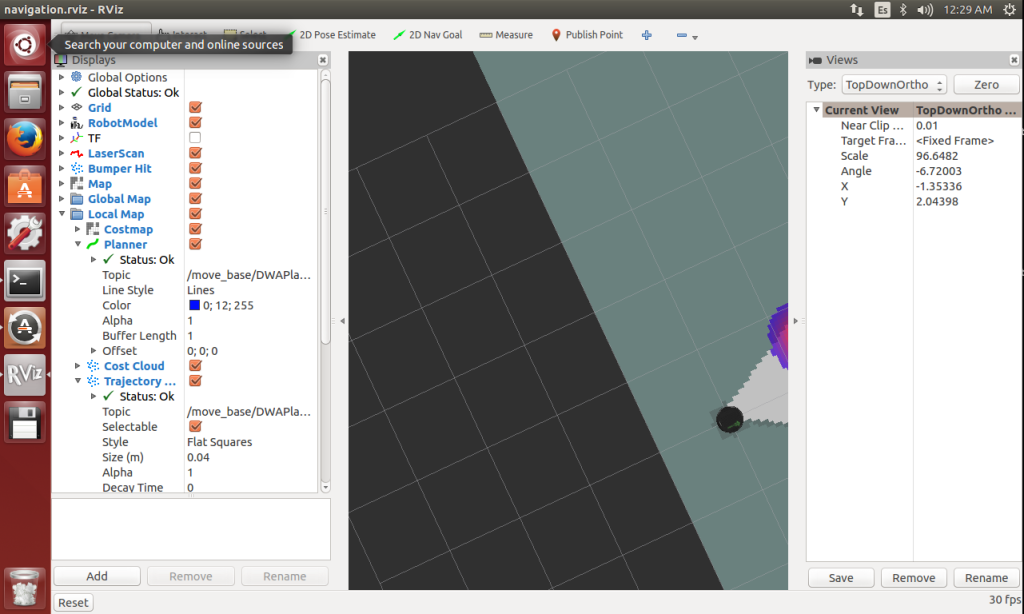
If RVIZ crashes on launch then launch it again and it will likely work (open source sucks sometimes). You should get a screen something like this:
If you don’t, or if you see “stop” signs in the column on the left then start troubleshooting. I usually begin by looking at the logs in the three terminal windows opened onto the robot. Critical messages are shown in red. A low battery is often the root of all evil.
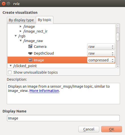
Assuming this has worked, close the “Views” frame on the right as it contributes nothing. You might want to add a video stream too. Click on the “Add” button bottom left, select the “By topic” tab, expand the /camera/rgb/image_raw topic and select “compressed” from the “Image” dropdown.
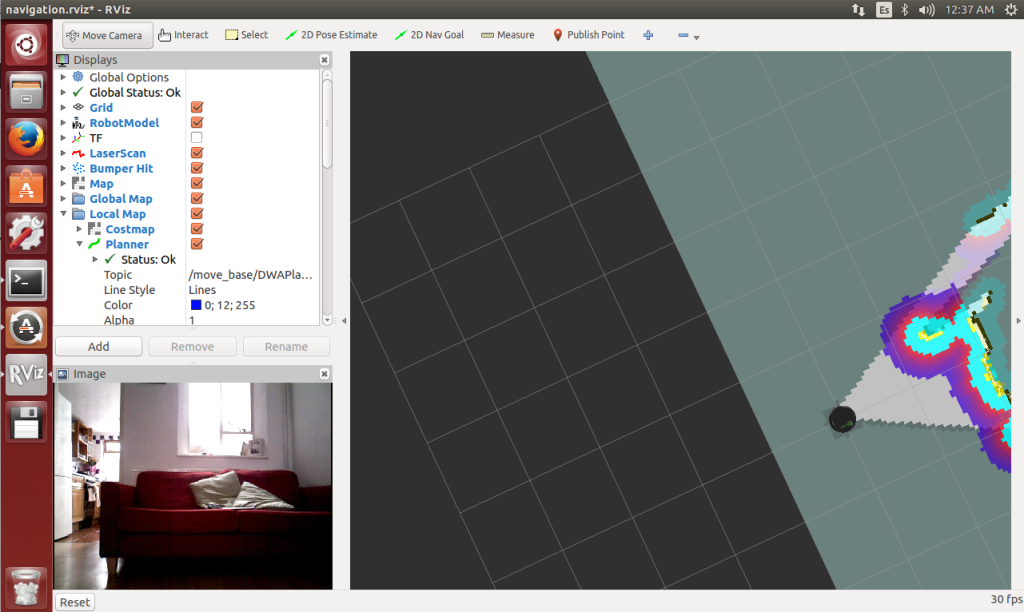
Click “Ok”. Now you should have a live video stream on the display. Adjust the relative sizes of the frames until you’re comfortable.
Personally, I find the Costmap confusing at this stage, so I disable it. Deselect the checkbox “Local map > Costmap”. You can rotate the display with the left mouse button, zoom in or out with the right mouse button and (most usefully) move the display with shift and the left mouse button.
What are we looking at here? This is a birds eye view of the map constructed so far. The robot is the black circle and we can see the walls or objects that the robot has located. The surrounding dark grey is unknown territory and the lighter colours represent space that the robot knows to be empty.
Where is this data coming from? Disable the items Map, Global Map and Local Map.
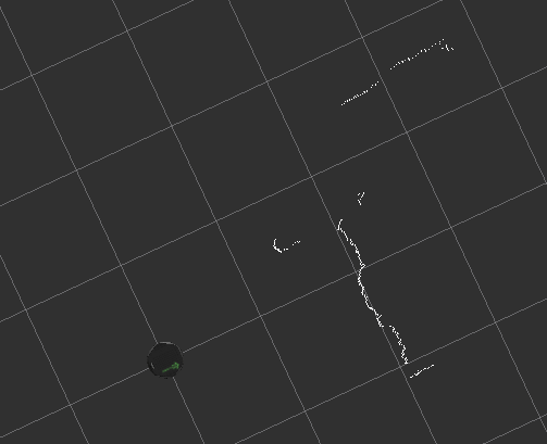
This is a little harder to see, but the white wiggly lines are the readings from the “laser scan”. This might seem odd, as the robot does not come equipped with a laser. In fact, the Xtion readings are being converted into a simulated laser scan, allowing the reuse of the navigation stack, which was built for LIDARs.
What this means in practise is that the only data being used from your Xtion is a thin horizontal slice of depth readings at the “eye-level” of the sensor. It’s not using the RGB pixel values, nor is it using the full set of depth information in the 2D viewport. This further means that the height you’ve positioned the sensor at determines what the robot thinks is on the “floor”. The map is a purely 2D map, a horizontal slice of the room at the height of the Xtion. This can cause problems with low objects which the system will miss entirely.
Re-enable the Map and Local Map. Now bring your “keyboard_teleop” terminal window into focus and navigate round the room with the keyboard to build up your complete map.
When you have a decent map, you’ll need to save it for later reuse. Open up a fourth shell into the robot and type:
rosrun map_server map_saver -f /home/ubuntu/my_map
Then quit RVIZ and close down the four terminal windows you opened onto the robot.
Autonomous Navigation
SLAM is something you do once, when you build up a map for the first time. Localization is something you need to do whenever the robot is moving. Now let’s use the map you constructed in an everyday scenario of autonomous navigation.
Shell into the robot and start the basic nodes again:
roslaunch turtlebot_bringup minimal.launch
Shell in with a second window and start AMCL, of which more in a minute:
roslaunch turtlebot_navigation amcl_demo.launch map_file:=/home/ubuntu/my_map.yaml
Check the log on this second window. You should eventually see the message “odom received!” which indicates that AMCL is working.
On the ROS workstation, fire up RVIZ with
roslaunch turtlebot_rviz_launchers view_navigation.launch --screen
Remove the Views pane and add back in the video streaming as described above.
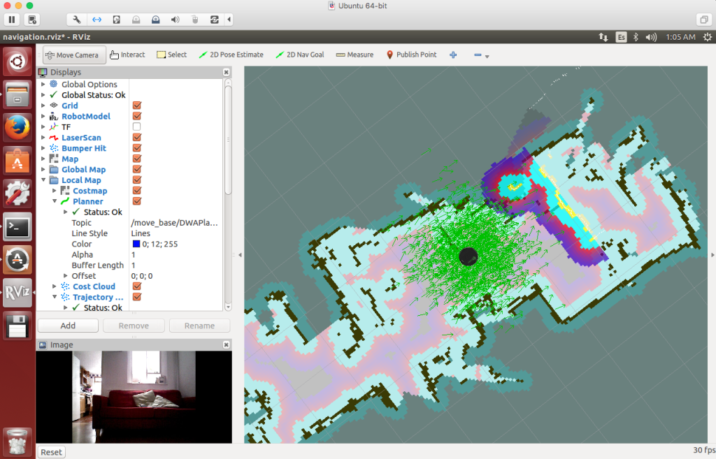
We can see the map that we created in the previous section as well as a “cost map” (the purple fringes). There’s also a green haze around our robot. Let’s take a closer look at it.
If you’ll recall, in order to perform the localization we code a probability function that gives us the probability that the robot is at any given point on the map, given the previous localization estimate, the map and some sensor readings:
probability of robot being at pose x at time t = p(robot pose at time t-1, sensor data, map)
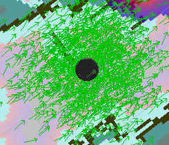
The green haze is a particle filter. This is a technique for finding the point of maximum probability over the entire map, without calculating the probability at every single (x,y) coordinate, which would be unreasonably slow. Actually, it would be every single (x, y, theta) where theta is the orientation of the robot; a pose on a 2D floor is actually three dimensional.
Instead of doing this potentially slow calculation every cycle, the AMCL (Adaptive Monte Carlo Localization) node makes a number of guesses of the robot pose, each one of which is known as a particle and each one of which is represented on the map by a green arrow showing the robot (x,y) and orientation theta.
Let’s say it maintains 1000 guesses or particles. On each cycle, for each particle, the code will work out the probability that the robot is actually there given the noisy sensor readings, the unreliable map and the previous best guess. The particle with the highest probability is the system’s best guess for the robot’s pose. It won’t be exactly the real location, but if the algorithm is well implemented, it will be close.
There are a number of variations of the algorithm that change how the guesses are chosen and updated. In general, poor probability guesses are culled from the list each cycle and are replaced with new guesses closest to the current best guess. As time goes on, the guesses should get better and better. Hence the “adaptive” in Adaptive Monte Carlo Localization. The “Monte Carlo” refers to the dice-rolling random element involved in making guesses.
The First 2D Pose Estimate
One more thing remains to be done, and at first glance it looks very much like cheating. Before navigating, we have to tell the robot where it is. What kind of lousy localization algorithm requires a human to to tell the robot where it is starting off?
The reason is that our probability function for time t requires a best guess from time t-1:
probability of robot being at pose x at time t = p(robot pose at time t-1, sensor data, map)
To get the very first robot pose at time t-1 we need the human operator to provide a guess. After that, the robot is on its own and should be able to keep track of where it is.
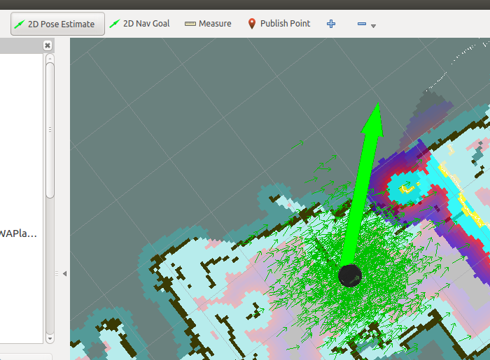
To do this, click on the button “2D Pose Estimate” and then on the map where you think your robot is. Drag the mouse pointer to show the direction you think your robot is facing (theta is just as important as its x,y coordinates).
In many cases your 2D Pose Estimate will coincide with where the robot model was already positioned. In other cases you’ll see the model and the particle filter cloud shift position.
There are many localization algorithms; some will require an initial estimate and others won’t. The first group won’t solve the kidnapped robot problem and the second will. The kidnapped robot problem is the difficulty a robot faces if it is suddenly kidnapped from a location it is certain of, blindfolded and then released in a new part of the map. Can it figure out its new location given that the pose at time t-1 was a long way away? AMCL doesn’t solve the kidnapped robot problem but works well if you refrain from kidnapping your robot, or turning it off and moving it.
At last, Navigation
Once localized with an initial 2D pose estimate, you should be able to navigate to your heart’s content.
Click on the button “2D Nav Goal” and select a point on the map where you want the robot to go. To start with, pick a position close to the starting point. Drag the mouse pointer to select the direction in which you want it to end up facing.
The robot will ponder, and then hopefully produce a planned trajectory to its goal, marked as a thin green line:
A number of things can go wrong at this point, so read the troubleshooting section below. If the planets are all in alignment, then your robot will rotate and trundle over to your goal.
Now pick a new goal and put the robot through its paces.
AMCL is robust to small or fleeting changes in the map. Try setting the robot along a path and then jumping in front of it. The robot should pause and navigate around you.
Troubleshooting
The AMCL algorithm is designed to be reliable despite noisy and changing environments. It’s therefore remarkable how often this simple demo seems to fail. Here are some of the root causes I’ve come across:
- Undercharged Kobuki battery (mentioned above)
- Wrong nodes running on the robot (operator stupidity)
- Time synchronization issues
- “Room” changed radically since map saved (e.g. by changing the vertical positioning of the Xtion)
- Trying to navigate through gaps that are too narrow for a robot that lacks self confidence.
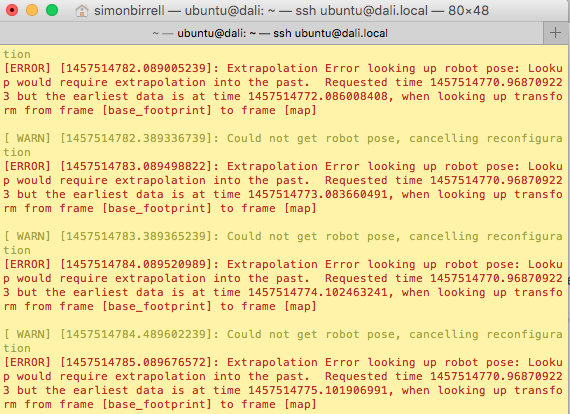
If the system clocks and dates are not aligned on the robot and ROS Workstation then you will likely see time synchronisation issues. You may see logs in the AMCL window like this:
The “Extrapolation Error looking up robot pose: Lookup would require extrapolation into the past” error is caused by a mismatch between the clocks on the robot and the ROS Workstation. To solve these
- Compare dates on the ROS Workstation and the robot. Type
dateon each device. To correct one or both of them, use
date -s '2016-3-25 12:34:56' - Do a fine-grained synchronisation on both devices to an external time server. Type
sudo ntpdate ntp.ubuntu.comThe very first time you do this you will need to install chrony, with
sudo apt-get install chrony
The final problem listed above is when you try to navigate through too narrow a gap. This is an interesting one, and brings us to cost maps. On the RVIZ display you should see an option to display the Costmap. Enable it, if it isn’t enabled already.
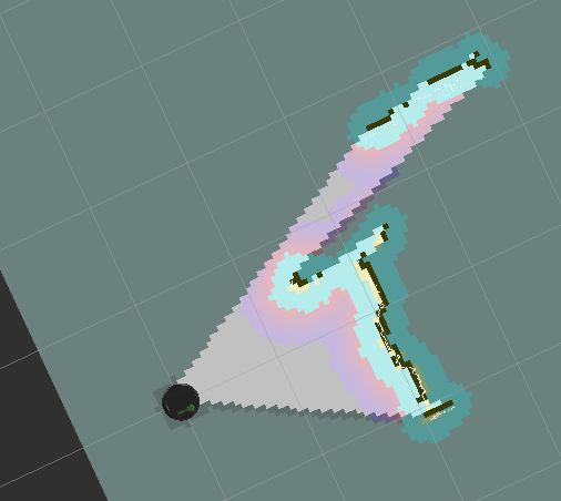
The costmap is visualised as a square round the robot containing the purple-fringed blobs. The colour represents the estimated cost for the robot of moving to the location. Going into walls is hard, but also going close to them might be hard too, given the uncertainty that surrounds the map and the robots position. So the robot leaves a safe zone round detected objects, and this is reflected in the cost map.
In the diagram above, the purple fringes are almost touching although the gap between the TV and the crib is actually perfectly large enough for the robot to get through. Any closer, and the robot will stubbornly refuse to go through.
The best way to find this kind of problem is to monitor the log messages in the AMCL window and read them carefully.
Wrap Up
We have built a map for the robot using manual navigation. We could then use the map to allow autonomous navigation using RVIZ as a user interface.
All of this will take some practise and tuning to get it working correctly in your environment. For a “solved problem”, it’s surprising how much fiddling you need to do to get it to work. Hopefully these instructions will help, but it makes you wonder about projects to run self-driving cars off ROS. I’m not sure I’ll be beta-testing those products.
All of this can potentially be controlled from code. You could write a Python ROS node to do the initial map building and another to send desired navigation points to the navigation stack for autonomous navigation.
